The tent map: implementation

Epilogue #

This was written way back in June 2023, fifteen months before I write this now. I do not plan to finish this blog; that being said, I’ve decided it’s better to have it up in its incomplete state than stuck in the drafts forever. Feel free to give it a read!

Background #

The tent map is a simple-to-implement example of a dynamical system with chaotic behavior, which makes it great as a toy example to mess with in code. The equation, here taken from Wikipedia, can be written either all as one or piecewise:

$$f_\mu(x) = \mu \min(x, 1-x)$$

$$f_\mu(x) = \begin{cases} \mu x & \text{if }x < \frac{1}{2} \newline \mu(1-x) & \text{if }x \geq \frac{1}{2} \end{cases}$$

The tent map is an example of a dynamical system which evolves by repeatedly applying a function. We set a starting point \(x_0\), apply \(f_\mu\) to it over and over, and study the sequence \([x_n]\) the process generates. Each element \(x_k\) of that system is equal to applying \(f_\mu\) a number of \(k\) times to \(x\), so the sequence looks like $$[x_n] = [x_0, f_\mu(x_0), f_\mu(f_\mu(x_0)), \dots]$$

Thinking of the indices in the sequence as timesteps, we’ve defined a discrete-time dynamical system from a starting value \(x_0\) with an evolution function \(f_\mu\).¹ This sequence may be more familiar as a recurrence relation where \(x_{n+1} = f_\mu(x_n)\), or could be interpreted as a discrete-time Markov chain. The great thing about math is that all of those interpretations are correct, which expands our toolbox and the questions we can explore.

To have a dynamical system this way, we need a phase space to track points in; additionally, it’s convenient if that phase space is bounded and if the points inside it are bounded to the space. That way, we can track how points evolve within a set space and not worry about a sequence falling outside of that space into undefined territory after some number of iterations. That desired bound is done here by restricting the points we put in to \(x\in [0, 1]\) and restricting our dynamical parameter to \(\mu\in (0, 2]\), so the function maps the unit interval to itself.

Naive coding approach #

So how do we simulate a discrete-time dynamical system using the tent map? Pretty easily:

import numpy as np

def tent_map_seq(start, n=100, mu=2):
    tent_map = lambda x: np.amin([x, 1-x]) * mu
    arr = np.zeros(n)
    arr[0] = start
    for i in range(n-1):
        arr[i+1] = tent_map(arr[i])
    return arr

import numpy as np

def tent_map_seq(start, n=100, mu=2):
    tent_map = lambda t, x: np.amin([x, 1-x]) * mu
    return np.array([start] +
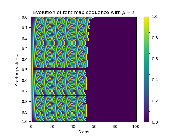
        [start := tent_map(t, start) for t in range(n-1)])

Now that we have a working implementation (in four lines, no less!), we can start exploring its dynamics—wait a minute, who said this actually works? It’s fast, and it does match up with the definition, but recall that the tent map has chaotic behavior, which means that by definition it is highly sensitive to initial conditions. So this is only guaranteed to work if we have infinite precision on our calculations. Indeed, we can make a graph showing the evolution of the tent map for a range of input values, and if we make one with this code, this happens:

Every input value becomes zero after only about 55 to 60 steps at max. If any value hit 1, that would make sense: 1 maps to 0, and 0 maps to itself. (In other words, 0 is a fixed point of the system.) But 0.4 shouldn’t ever hit zero; it should repeat in the cycle [0.4 -> 0.8 -> 0.4…] forever. (In fact, setting \(\mu = 2\) is a particularly nice example, since it can be shown that every rational point has periodic behavior over a sufficiently long period of time. Sufficiently long enough that if we go fine enough, it’ll look random in the amount of steps ran.)

At first, I didn’t realize a lack of precision would be an issue. But, after I ran the graph for the first time and this image came up, it reminded me of the issues I had on a past research project where roots of polynomials seemed to disappear. Floating-point error, in that case, was messing with Mathematica’s root-finding algorithm, and here, it was introducing small errors that compounded to erase long-term behavior.

Precise computation #

To fix this, we can restrict our view to the rational numbers. This doesn’t mean skipping values; finite-precision numbers are necessarily rational, so we were always limited to the rationals. What we can do, instead, is represent each number in fractional form as a pair of integers, and separately calculate the effects of the map on the numerator and denominator. Only working with integers means we never need to worry about floating point error, only overflow.² Denote \(\mu = \frac{\mu_1}{\mu_2}\) so \(\mu\) is a rational as well, and then

$$ \frac{p}{q} < \frac{1}{2} \iff 2p < q$$

$$f_\mu\left(\frac{p}{q}\right) = \begin{cases} \frac{\mu_1 p}{\mu_2 q} & \text{if }2p < q \newline \frac{\mu_1(q-p)}{\mu_2 q} & \text{if }2p \geq q \end{cases}$$

This is, once again, simple to implement. Make a lambda function, this time taking in a list of two numbers, and sweep through and array to build up the sequence.

def tent_map_rational_sequence(start=[1, 2], n=100, mu=[1, 1]):
    fmu = lambda lst: [np.amin([lst[0], lst[1]-lst[0]]) * mu[0], lst[1] * mu[1]]
    arr = np.zeros((n, 2))
    arr[0] = start
    for i in range(n-1):
        arr[i+1] = fmu(arr[i])
    return np.divide(arr[:, 0], arr[:, 1])

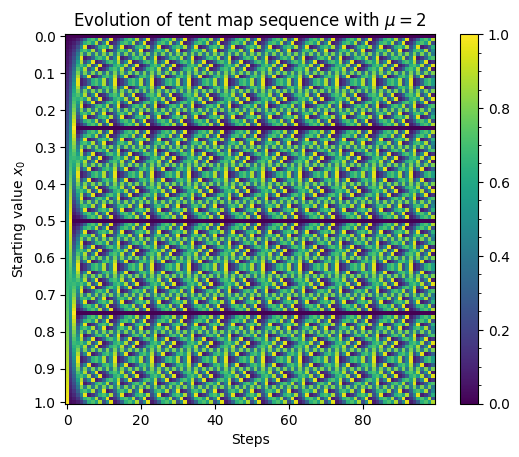
Graphing this time shows that we no longer suffer from floating-point errors, as the pattern continues infinitely: